Semantic Search Tutorial

A full semantic search tutorial about:

• data mining with requests and beautifulsoup
• preprocessing in pandas
• chunking the document text in smaller paragraphs of the right size for the ML model
• creating embeddings for each chunk
• calculating the mean embedding for each document
• saving data as gzipped json (small file size & easy and fast to read in js with pako.js)
• creating a static web app based on transformers.js on GitHub Pages

App here

Intro

For the past decades, full-text search aka keyword-based search was the dominating search method for the web. Thanks to the recent uprise of quantized machine learning (ML) models and easy-to-use tools in Python for processing and JavaScript for hosting a model it has become easier than ever to create a semantic search engine yourself and host it as a static web app for free on GitHub Pages.

This tutorial guides you through the steps of the Jupyter Notebook. You could run it on Colab but it should work just as well locally on Ubuntu, Mac and Windows. No GPU needed - your average laptop will handle the workload just fine!

Foreword: Guerilla Semantic Search

There are plenty of web apps and dashboards, interfaces, or databases out there that just offer full-text search when semantic search could add a lot of value to the end users. It’s especially evident in the scientific field, where you frequently encounter domain-specific terminology that researchers from other disciplines may not be familiar with. A full-text search would be ineffective unless some preliminary research into the field is conducted to identify the essential keywords needed for full-text search.

The big advantage of semantic search is that it searches not for key terms but instead for the meaning. E.g. when you’re researching “urban heat islands” - a particular phenomenon where urban areas become significantly hotter than rural areas - but you maybe never heard of the term before you can simply search for “hot temperatures in cities” and semantic search will yield the right results.

I want to coin a term here with this tutorial, when mining data from existing full-text search apps, indexing the data and providing an interface to perform semantic search. Let’s call it - sarcastically - Guerilla Semantic Search. It kind of catches the spirit of an independent movement quickly taking on full-text search instead of simply waiting for change. It’s basically thought as an interim solution until the original web page adopts semantic search too.

Tutorial

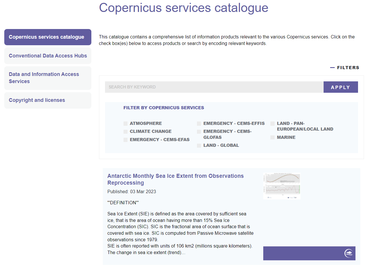
We’ll use the Copernicus Services Catalogue here as example. The Copernicus program as “Europe’s eyes on earth” is

“[…] offering information services that draw from satellite Earth Observation and in-situ (non-space) data.” (Source: https://www.copernicus.eu/en/about)

The Copernicus Services Catalogue is a crucial interface for researchers, providing access to the different services’ metadata of:

• atmosphere
• marine
• land
• climate change
• security
• emergency

As of October 2023, it is limited to the classic “search by keyword” functionality and offers just a service filter - perfect for this tutorial!

1 Data Mining

1.1 Mining the URLs

Let’s understand how the site works first. There is some kind of title (even though it’s a little cryptic) and a description teaser (that looks like there are some JSON/DB formatting errors with additional quotes). Each of the tiles holds a hyperlink to the full metadata. Unfortunately, the site does not provide any kind of API and does not load a JSON file we could use. So we’ll stick with classic web scraping.

But how many entries are there overall? The pagination doesn’t help…

If you go the last page and then one page back to page 46 to count the results and multiply it with the number of pages you’ll get confused as the CSS is terribly broken.

Let’s go one more page back to page 45 and count the elements there: it’s 18 entries. Multiplied by 46 that makes for 828 entries + 6 entries from the last page, ergo 834 entries. Great - now we have a reference point when scraping the URLs!

As we cannot modify the number of results per page, we need to fire 47 requests, loading each page.

Mining the data is fairly straight forward:

 1
 2
 3
 4
 5
 6
 7
 8
 9
10
11
12
13
14
15
16
17
18
19
20
21
22
23
24
25
26
27
28
29
30
31
32
33
34
35
36
37
38
39
40
41
42
43
44
45
46
47

import requests
from bs4 import BeautifulSoup
import pandas as pd
import time 
from tqdm import tqdm

base_url = "https://www.copernicus.eu/en/accessing-data-where-and-how/copernicus-services-catalogue?page="
start_page = 0
end_page = 49 # Can be more than available, makes no difference

# Create an empty list to store data
data_list = []

for page in tqdm(range(start_page, end_page + 1)):
    time.sleep(2)
    url = base_url + str(page)
    response = requests.get(url)

    if response.status_code == 200:
        # Parse the HTML content
        soup = BeautifulSoup(response.text, 'html.parser')

        # Find the <div> with the specified classes
        div_with_classes = soup.find("div", class_="col-12 mb-2 media-articles service-catalogue-articles")

        if div_with_classes:
            # Find all <a> elements within the specified <div>
            a_elements = div_with_classes.find_all("a")

            # Extract and append links that start with "/en/access-data/"
            for a in a_elements:
                href = a.get("href")
                if href and href.startswith("/en/access-data/"):
                    full_url = url
                    data_list.append({"Page Number": page, "Page_URL": full_url, "Link": href})
        else:
            print(f"No <div> with specified classes found on page {page}")
    else:
        print(f"Failed to fetch data from page {page}. Status code: {response.status_code}")

# Convert the list of dictionaries to a Pandas DataFrame
df = pd.DataFrame(data_list)
df["Service_URL"] = "https://www.copernicus.eu" + df["Link"]
del df["Link"]

df.to_csv("copernicus_services_october-2023.csv.gz", compression="gzip", encoding="utf-8", index=False) # save intermediate file as backup
print("Done!")

This will create the initial dataframe with 834 entries - perfect, exactly the number we expected!

1.2 Mining the titles and descriptions

The individual pages always follow the same pattern, e.g. this page. They consist of:

• a title (unfortunately sometimes a little cryptic)
• a description (important for indexing later!)
• the catalogue URL to the product
• the service category (e.g. land, marine etc.)
• a last updated datetime object

If you open the individual pages in the browser you will note, that when the content exceeds a certain amount of words, it will be hidden and a “read more” button will be displayed. Luckily, this is done via external JavaScript that is executed on page load so that when the Python request receives the HTML all content is included! Else it would have been problematic and we’d have to use Selenium or other tools to perform a “click” on the page.

For the purpose of this tutorial we’ll keep it simple and just mine the title, description and catalogue URL.

Iterate over the individual pages:

 1
 2
 3
 4
 5
 6
 7
 8
 9
10
11
12
13
14
15
16
17
18
19
20
21
22
23
24
25
26
27
28
29
30
31
32
33
34
35
36
37
38
39
40
41
42
43
44
45
46
47
48
49
50
51
52
53
54
55
56
57
58
59
60
61

import requests
from bs4 import BeautifulSoup
import pandas as pd
import re  # Import the re module for text processing
from tqdm import tqdm

# Load the initial DataFrame from your CSV file
df = pd.read_csv("copernicus_services_october-2023.csv.gz")#.head(10)

# Create empty lists to store extracted data
titles = []
content_text = []
mx_auto_links = []

# Define a function to remove triple quotes from text
def remove_triple_quotes(text):
    return re.sub(r"'''", "", text)

for index, row in tqdm(df.iterrows()):

    time.sleep(2) # be gentle and add 2 seconds of break for each iteration!
    url = row["Service_URL"]
    response = requests.get(url)

    if response.status_code == 200:
        # Parse the HTML content
        soup = BeautifulSoup(response.text, 'html.parser')

        # Extract the main content <div> with the specified class
        main_content_div = soup.find("section")

        if main_content_div:
            # a) Extract h3 element (Title)
            h3_element = main_content_div.find("h3")
            title = h3_element.text if h3_element else "N/A"
            titles.append(title)

            # b) Extract visible text content from div with class "ec-content" and its children
            ec_content_div = main_content_div.find("div", class_="ec-content")
            content = " ".join([remove_triple_quotes(tag.get_text()) for tag in ec_content_div.find_all(True)]) if ec_content_div else "N/A"
            content_text.append(content)

            # c) Extract all href elements in div with class "mx-auto mt-5"
            mx_auto_div = main_content_div.find("div", class_="mx-auto mt-5")
            mx_auto_links_div = mx_auto_div.find_all("a") if mx_auto_div else [""]
            mx_auto_links.append([link.get("href") for link in mx_auto_links_div][0])
            
        else:
            print(f"No content <div> found on page {row['Page Number']}")

    else:
        print(f"Failed to fetch data from page {row['Page Number']} {row['Service_URL']} - Status code: {response.status_code}")

# Add the extracted data to the DataFrame
df["Title"] = titles
df["Content"] = content_text
df["Catalogue_URL"] = mx_auto_links

df.to_csv("copernicus_services_title_descr_url_october-2023.csv.gz", compression="gzip", encoding="utf-8", index=False)

print("Done!")

If some iterations might fail, you can check manually whether these pages contain errors. If they don’t either the server or your internet connection might be unstable. You can always add entries manually or re-run the script in this case. For me, everything went fine without errors - note that I also included a break of 2 seconds for each iteration.

2 Document chunking

Let’s first take a look at the distribution of description length. Pandas offers a built-in histogram function:

1
2
3
4
5

import pandas as pd
df = pd.read_csv("copernicus_services_title_descr_url_october-2023.csv.gz")
df["Content_Length"] = df.Content.apply(lambda x: len(str(x)))
df = df.sort_values("Content_Length")
df[df['Content_Length'] < 4000].Content_Length.hist(bins=1000) # cutoff as there is only one entry with an extremely long content length

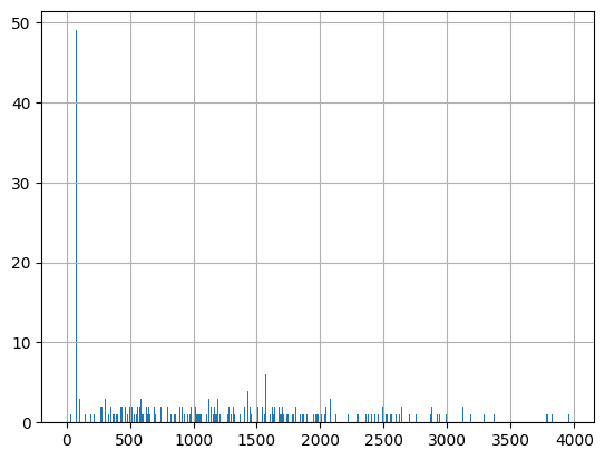
It seems that there are a few documents that have little or now description but the rest is ranging somewhere between 500 and 3000 characters. Looking closer at the data the peak of ~50 documents shows descriptions indicating that there is no description. You can clean the dataframe but if it’s only for semantic search, you could also leave it as is since these results wouldn’t show up anyway.

Now that we have a dataframe with title, content and URLs we can start and index the data!

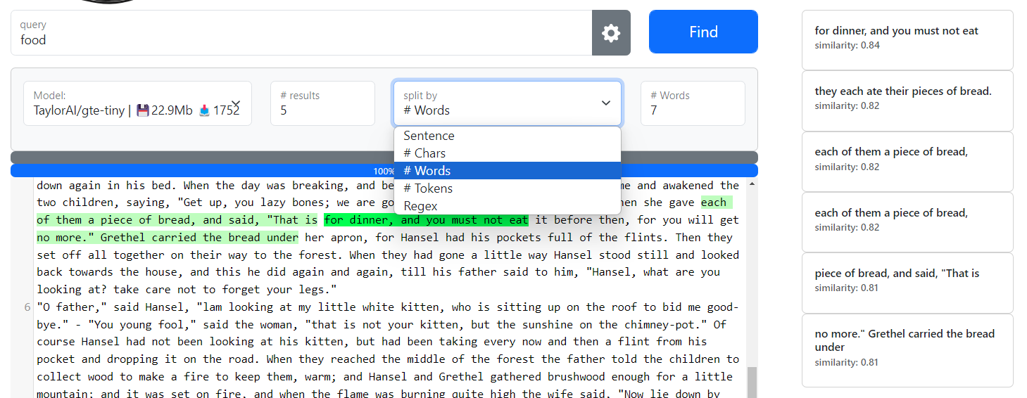
We will use the Haystack Python framework to chunk our content as it provides some convenience functions. You could however, just as well write a custom chunking function based on paragraphs, sentences, words, characters or a regex similar to what you find on SemanticFinder - try it out to see how the chunking affects the results!

But why do we need to chunk our data at all? The problem is that LLMs or the smaller versions we are using in this tutorial have a limited context length they can process. In other words, they can only digest a few sentences at once - the rest would be cut off and ignored otherwise. To be precise, the context length is not expressed in words or sentences but rather in tokens. We can count the tokens ourself:

1
2
3
4
5
6
7
8

from transformers import AutoTokenizer
tokenizer = AutoTokenizer.from_pretrained('sentence-transformers/all-MiniLM-L6-v2')
def token_num(sentence):
    tokens = tokenizer.tokenize(sentence)
    return len(tokens)

token_num("test this tokenizer")
# 4 tokens

Use the OpenAI tokenizer to estimate tokens; their rule of thumb is as follows:

A helpful rule of thumb is that one token generally corresponds to ~4 characters of text for common English text. This translates to roughly ¾ of a word (so 100 tokens ~= 75 words). (Source: https://platform.openai.com/tokenizer)

We need to tune the content length we pass to the ML model in a way that it’s as long as possible but not cutting of any content. With haystack we can test and find just the right number of words by e.g. looking at the largest content length in our dataframe with df.iloc[657] and experimenting with the split_length:

 1
 2
 3
 4
 5
 6
 7
 8
 9
10
11
12
13
14
15
16
17
18
19
20

from haystack.nodes import PreProcessor # python 3.9.1. works
processor = PreProcessor(
    clean_empty_lines=True,
    clean_whitespace=True,
    clean_header_footer=True,
    remove_substrings=None,
    split_by="word",
    split_length=60, # attention: might cut off large table content or similar. Watch out for model max token input!
    split_respect_sentence_boundary=False,
    split_overlap=0,
    max_chars_check=1000000,
    show_progress_bar=False
)

res = processor.process([{'content': df.iloc[657].Content}])

a = [i.to_dict()["content"].strip() for i in res] 

[token_num(i) for i in a]
# [71, 83, 74, 87, 81, 110, 113, 116, 80, 77, 81, 76]

The aim here is not to exceed 128 tokens for sentence-transformers/all-MiniLM-L6-v2 but get as close as possible. If you’d like to use another model from the MTEB leaderboard like the gte or bge models that yield better results than Sentence Transformers, be sure to check the max token length before.

3 Document indexing

Ok, let’s define a helper function for mean embeddings and test it:

 1
 2
 3
 4
 5
 6
 7
 8
 9
10
11
12
13
14
15

import torch 

def mean_embedding(in_vectors):
    try:
        return list(torch.mean(torch.tensor(in_vectors),dim=0).numpy())
    except Exception as e:
        print(e)
        return []

mean_embedding([
    [0.17, 0.2, 0.3, 0.4],
    [0.2, 0.3, 0.4, 0.5],
    [0.3, 0.4, 0.5, 0.6]])

# [0.22333334, 0.29999998, 0.4, 0.5]

The function we apply to the dataframe does a few things:

• chunks the content
• calculates the embedding for each chunk with sentence-transformers/all-MiniLM-L6-v2
• calculates the mean embedding for the document

 1
 2
 3
 4
 5
 6
 7
 8
 9
10
11
12
13
14
15

from sentence_transformers import SentenceTransformer
model = SentenceTransformer('sentence-transformers/all-MiniLM-L6-v2')

def text_to_embedding(in_text):
    res = processor.process(
        [
            {
                'content': in_text
            }
        ]
    )

    a = [i.to_dict()["content"].strip() for i in res] #res[0].to_dict()

    return mean_embedding([model.encode(i) for i in a])

Let’s add a null vector to each row by default and overwrite them with the real mean embedding if the content is not empty:

1
2
3
4

df = df.fillna(" ")
null_vector = [0] * 384
df["mean_embedding"] = df.Content.apply(lambda x: null_vector)
df.loc[df.Content != " ", "mean_embedding"] = df.loc[df.Content != " ", "Content"].progress_apply(lambda x: text_to_embedding(x)) # 13 min!

The indexing of all 834 entries took me 13 minutes on my old i7 laptop running entirely on CPU.

Let’s export the resulting dataframe to a gzipped json. That’s now exactly the file being loaded on the final web app:

1

df[['Service_URL','Catalogue_URL','Title', 'Content', 'mean_embedding']].to_json("copernicus_services_embeddings.json.gz", compression="gzip", orient="records")

4 Test search

You can run some test search on your dataframe right in Jupyter. Define a cosine similarity function, set a larger column output size for pandas columns and calculate the cosine similarity score for each row:

 1
 2
 3
 4
 5
 6
 7
 8
 9
10
11
12
13
14
15

pd.set_option('display.max_colwidth', 200)
import torch.nn.functional as F

user_query_embedding = model.encode("arctic")

def cosine_sim(embedding1, embedding2):
    embedding1 = torch.tensor(embedding1, dtype=torch.float32)
    embedding2 = torch.tensor(embedding2, dtype=torch.float32)
    cosine_similarity = float(F.cosine_similarity(embedding1, embedding2, dim=0))
    similarity_score = 0.5 * (cosine_similarity + 1)
    return similarity_score

df["similarity_score"] = df.mean_emebdding.apply(lambda x:cosine_sim (user_query_embedding, x) )
df = df.sort_values("similarity_score", ascending=False)
df.head(5).Content

It will output these columns:

1
2
3
4
5

55     Short description:\nArctic Sea and Ice surface temperature  Detailed description:\nArctic Sea and Ice surface temperature product based upon reprocessed AVHRR, (A)ATSR and SLSTR SST observations f...
56     Short description:\nArctic Sea and Ice surface temperature  Detailed description:\nArctic Sea and Ice surface temperature product based upon reprocessed AVHRR, (A)ATSR and SLSTR SST observations f...
589    DEFINITION Net (positive minus negative) volume transport of Atlantic Water through the sections (see Figure 1):  Faroe Shetland Channel (Water mass criteria, T > 5 °C); Barents Sea Opening (T > 3...
707    DEFINITION Net sea-ice volume and area transport through the openings Fram Strait between Spitsbergen and Greenland along 79°N, 20°W - 10°E (positive southward); northern Barents Sea between Svalb...
54     Short description: Arctic Sea and Ice surface temperature product based upon observations from the Metop_A AVHRR instrument. The product is a daily interpolated field with a 0.05 degrees resolutio...

Looks good to me!

Web app

A high-level overview of what’s happening in the web app:

• load the ML model and the data dump (gzipped json)
• user inputs a query
• an embedding is calculated
• for every of the 834 documents in our JSON, the similarity score is calculated. It’s a simple vector operation so it’s very fast and the calculation time is so low, it seems to be instant
• the results are sorted by highest similarity score (very fast too)
• for the top N results, the items are appended to the HTML table and rendered properly (hyperlinks, “read more” button etc.)

Note that I intentionally kept it as simple as possible and avoided package managers, TypeScript, ES6, frontend frameworks etc. It’s just plain JavaScript in one file you can easily modify. If you want to go that way too just keep in mind that:

• you need to use an older version of transformers.js running without ES6
• for larger apps the UI might freeze (however not noticeable here); avoidable with new transformers.js version and web workers
• if your project grows in complexity, definitely consider using ES6 to separate the JS
• using npm for JS packages has plenty of advantages and webpack outputs you a cleaner and smaller build

1 Loading a gzipped JSON

We exported the data as a gzipped json with .to_json("copernicus_services_embeddings.json.gz", compression="gzip", orient="records") so it saves disk space and can be loaded faster. As it’s only 2.5Mb there is no real need to put much effort in reducing the file size. You could however use product quantization or simply reduce the decimals, but that’s content for another tutorial!

The gzipped json can be loaded with pako.js in a few lines of JS:

1

<script src="https://cdnjs.cloudflare.com/ajax/libs/pako/2.1.0/pako.min.js"></script>

 1
 2
 3
 4
 5
 6
 7
 8
 9
10
11
12
13
14
15
16
17
18
19
20
21
22
23
24
25
26
27

let copernicus_services

function fetchUnzip(url){
    fetch(url=url)
        .then((response) => {
            if (!response.ok) {
                throw new Error('Network response was not ok');
            }
            return response.arrayBuffer(); // Get the response as an ArrayBuffer
        })
        .then((gzippedData) => {
            // Decompress the gzipped data using pako
            console.log("file loaded, start decompression");
            const jsonString = pako.inflate(new Uint8Array(gzippedData), { to: 'string' });

            // Parse the JSON string into an object
            const jsonObject = JSON.parse(jsonString);

            // Callback with the extracted JSON object
            console.log("file decompressed");
            copernicus_services = jsonObject
            return jsonObject;
        })
        .catch((error) => {
            console.error('Error loading or extracting JSON.gz:', error);
        });
}

I also tried a fancier way with DuckDB-Wasm and loading potentially faster parquet files but I eventually gave up as it turned out to be too complicated. Also it required ES6 logic which I wanted to avoid here.

The heart of the web app is transformers.js allowing you to run a quantized (=reduced in size) version of the model we use here right in your browser without GPU: sentence-transformers/all-MiniLM-L6-v2. I choose it as it is one of the smallest quantized models with around 24Mb of size, see here. Now, only gte-tiny is comparable in size and yields slightly better results.

2 Calculating embeddings with transformers.js

1

<script src="https://cdn.jsdelivr.net/npm/@xenova/transformers@1.4.3/dist/transformers.min.js"></script>

The old version of transformers.js uses an asynchronous function to calculate the embedding:

1
2
3
4
5
6
7
8
9

let pipe
let currentQueryEmbedding

async function main() {
    pipe = await pipeline("embeddings", "sentence-transformers/all-MiniLM-L6-v2");
}

let output = await pipe(inputText);
currentQueryEmbedding = output.data

You can clone this repo and use it as template for other projects. Hosting the web app on GitHub Pages is free.

3 Cosine similarity

Calculating the cosine similarity score for between the user query embedding and each of the 834 documents is quite simple:

1
2
3
4
5
6

function cosineSimilarity(vectorA, vectorB) {
    const dotProduct = vectorA.reduce((acc, val, i) => acc + val * vectorB[i], 0);
    const magnitudeA = Math.sqrt(vectorA.reduce((acc, val) => acc + val ** 2, 0));
    const magnitudeB = Math.sqrt(vectorB.reduce((acc, val) => acc + val ** 2, 0));
    return dotProduct / (magnitudeA * magnitudeB);
}

Note however, that this function can be sped up massively by pre-calculating the user query embedding magnitude once only instead of 834 times! So we change the function accordingly:

 1
 2
 3
 4
 5
 6
 7
 8
 9
10
11
12
13
14
15
16
17
18
19
20
21
22
23
24
25
26
27
28
29
30

let currentQueryEmbeddingMagnitude

function cosineSimilarity(vectorA, vectorB) {
    const dotProduct = vectorA.reduce((acc, val, i) => acc + val * vectorB[i], 0);
    const magnitudeB = Math.sqrt(vectorB.reduce((acc, val) => acc + val ** 2, 0));
    return dotProduct / (currentQueryEmbeddingMagnitude * magnitudeB);
}

function calculateSimilarity(currentQueryEmbedding, jsonData) {

    currentQueryEmbeddingMagnitude = Math.sqrt(currentQueryEmbedding.reduce((acc, val) => acc + val ** 2, 0));

    // Calculate similarity scores for each entry in jsonData
    const similarityScores = jsonData.map(entry => ({
        Service_URL: entry.Service_URL,
        Catalogue_URL: entry.Catalogue_URL,
        Title: entry.Title,
        Content: entry.Content,
        //mean_embedding: entry.mean_embedding, // not needed in the html table afterwards
        similarity: cosineSimilarity(currentQueryEmbedding, entry.mean_embedding),
    }));

    // Sort the entries by similarity in descending order
    similarityScores.sort((a, b) => b.similarity - a.similarity);

    // Return e.g. the top 20 entries
    const topResults = similarityScores.slice(0, 20);

    return topResults;
}

Further ideas

In order to keep this project a weekend project I neglected a few things that might be worth considering in the future, namely:

• code optimization and clean-up
• improving the UI and adding support for mobile devices
• comparing product quantization to simply reducing float decimals for smaller file sizes
• using DuckDB to use arrow data structure and parquet file format
• adding hybrid search, a combination of traditional full-text search and semantic search
• comparing the results of different small models (though very easily done with SemanticFinder)
• directly highlighting the most related text fragments on the page like the Chrome extension of SemanticFinder

Conclusion

You can easily mine data and process it with Python thanks to beautifulsoup, PyTorch, Haystack and transformers. Creating the semantic search web app requires a few tricks but this tutorial should provide you with the basics to get started with your own app!

It’s a very valuable effort for anyone who really needs to find just the right document. Let me know if this tutorial was helpful or if you even managed to create your own app! Tag me on Twitter/X, Mastodon or LinkedIn - always happy to hear from you. :)

P.S. For the seasoned web devs here: we are looking for contributors for SemanticFinder!