Using Jupyter Notebook as GIS

Clipping a geodataframe and displaying it on a basemap in Jupyter.

Loading a geodataframe

Let’s load some points from a geojson file, i.e. from our preprocessed geodataframe mined with Fast Instagram Scraper:

import geopandas as gpd
gdf = gpd.read_file("some_points.geojson")
gdf

Clipping a geodataframe with another…

If we would like to clip these points to the extent of a city, geopandas.clip method is pretty straightforward. Note that geopandas can read a file directly from URL as well! Here we load a geojson file of the extent of Bonn.

bonn = gpd.read_file("https://stadtplan.bonn.de/geojson?Thema=21248") # Bonn geojson
bonn = bonn.to_crs("EPSG:3857") # reprojection needed
clipped = gpd.clip(gdf, bonn) # clip 
clipped

… or clipping by indexing coordinates

In case you don’t have an exact shape to clip for geodataframe, but want to quickly remove outliers, you can make use of geopandas.cx function. You can index coordinates and set a max or min latitude or longitude. First indexer is latitude, second longitude:

clipped = gdf.cx[:, :7.543662]
clipped

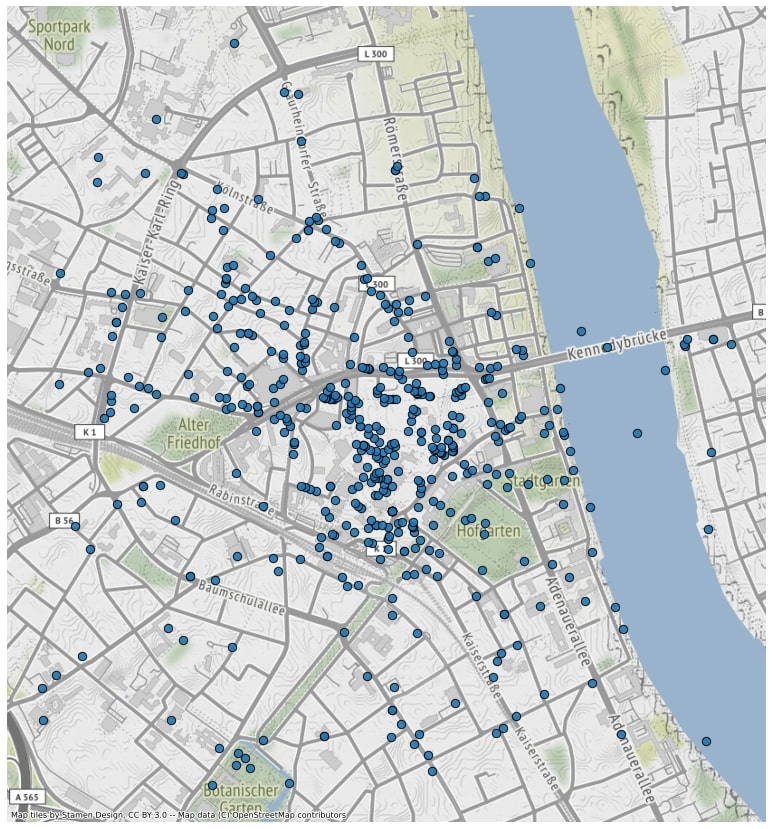
Plotting points on a basemap

%matplotlib inline

import matplotlib
import matplotlib.pyplot as plt
import geopandas as gpd
import contextily as ctx

ax = clipped.plot(figsize=(15, 15), alpha=0.9, edgecolor='k', markersize=70)
ctx.add_basemap(ax) # add zoom-level if needed i.e. zoom=12
ax.set_axis_off()

The result will look like this: