DuckDB for Geospatial

Using DuckDB for geospatial workflows for incredible performance boost! Leveling up my GeoPandas workflows for processing the 100M Foursquare dataset.

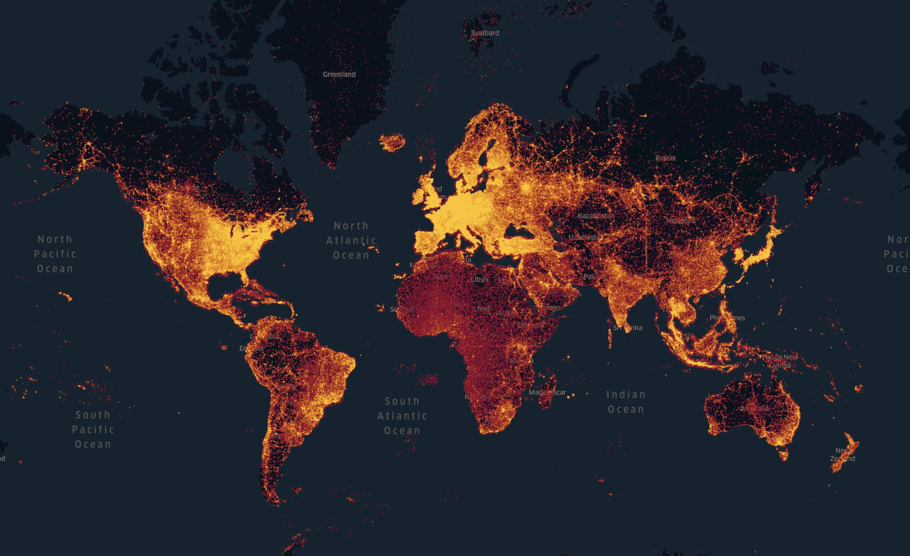
Image Source: Foursquare

This blog article, as my previous ones, have been written by myself. No GenAI was used except for improving code and doing research.

Motivation

The past two years were fantastic years for open data. Just to name a few fundamental releases:

1. Overturemaps: first non-beta dataset in 2024, now grown to more than >50.000.000 places https://overturemaps.org/

2. Foursquare: released >100.000.000 places in November 2024 https://docs.foursquare.com/data-products/docs/places-data-overview

3. EU High-Value Datasets Regulation (2023/138): in force since June 2024, finally forcing EU member states to open all kinds of datasets like parcel data, DOPs, DEMs/DSMs etc. Read through the annex what kind of spatial datasets to expect https://eur-lex.europa.eu/eli/reg_impl/2023/138/oj

With all three however, the challenge is data harmonization. Peaking at the category systems of Overturemaps (>2000 entries) and Foursquare (>1000) the question remains how to bring OSM and those two together.

For researchers like me, all three are valuable data sources and fit my research on geospatial semantic search perfectly! Especially Foursquare as a social-media-like dataset where users could write anything to “check in” somewhere in any language and with sentiments is perfect for my use case. So let’s dive in!

Performance Comparison: GeoPandas vs. DuckDB Spatial

Basic Example: Loading and String Filtering

I recently processed the entirety of more than 100.000.000 Foursquare places and created an httpfs-based data exploration workflow. That means that I provide a data dump on Huggingface (https://huggingface.co/datasets/do-me/foursquare_places_100M) as parquet file that you can explore and filter wihtout having to download everything. Instead, you can use DuckDB on your device and query the data remotely. The parquet file structure is quite advanced, so your DuckDB client will (almost) only pull the data needed.

For example, filtering the full 10Gb file remotely for all entries containing the word bakery, takes only 70 seconds on my setup. I’m using Python 3.11 here with duckdb installed.

import duckdb
duckdb.sql("INSTALL httpfs;LOAD httpfs;") # required extension
duckdb.sql(f"SELECT * FROM 'hf://datasets/do-me/foursquare_places_100M/foursquare_places.parquet' WHERE name ILIKE '%bakery%' ").df()

For convenience and better formatting I added a .df() at the end so the results get converted to a pandas df right away.

If instead you download the full file and query locally, the exact same query only takes 4.5 seconds!

import duckdb
duckdb.sql("SELECT * FROM 'foursquare_places.parquet' WHERE name ILIKE '%bakery%' ").df()

For comparison, only for loading this file, geopandas takes 2-3 minutes (!):

import geopandas as gpd
gdf = gpd.read_parquet("foursquare_places.parquet")

Filtering in geopandas then is fairly fast but expectedly much slower than DuckDB with 19 seconds:

gdf[gdf["name"].str.contains("bakery", case=False, na=False)]

Spatial Filters

Now, let’s use a spatial filter! Let’s say we’d like to export a file with only the locations in Germany. In GeoPandas, it’s straightforward, but the problem is that we first need to load the file and waste precious time again. Instead, let’s use DuckDB here. For simplicity, let’s take a hand-clicked file I created with https://geojson.io/#map=5.29/51.102/10.383.

{
    "type": "FeatureCollection",
    "features": [
      {
        "type": "Feature",
        "properties": {},
        "geometry": {
          "coordinates": [
            [
              [
                7.453920357277241,
                55.77849646824404
              ],
              [
                4.92271751197012,
                50.16986073820141
              ],
              [
                8.618720908704915,
                46.31228837218757
              ],
              [
                14.401005700128906,
                46.78989436018287
              ],
              [
                15.28371666973527,
                49.474039976208246
              ],
              [
                13.67006747473934,
                49.967381421377155
              ],
              [
                15.843708126034244,
                51.092067069612284
              ],
              [
                15.745164062426966,
                54.90592810042361
              ],
              [
                7.453920357277241,
                55.77849646824404
              ]
            ]
          ],
          "type": "Polygon"
        }
      }
    ]
  }

Now save this as germany.geojson in the working directory and run this code. The output is the filtered pandas df.

import duckdb
import geopandas as gpd
import pandas as pd
from shapely.geometry import Polygon

# Load the GeoJSON file and get the polygon for filtering
filter_poly = gpd.read_file("germany.geojson")
filter_poly.crs = "EPSG:4326"
polygon = filter_poly.iloc[0].geometry
polygon_wkt = polygon.wkt

# Define parameters
file_path = "foursquare_places.parquet"
n_lines = 110_000_000 # reduce lines for test runs
polygon_epsg = "EPSG:4326"  # EPSG code as a string

# Connect to DuckDB and load spatial extension
con = duckdb.connect()
try:
    con.execute("LOAD spatial;") # needs to be installed before with INSTALL spatial;
except Exception as e:
    print(f"Error loading spatial extension: {str(e)}")
    con.close()

# Construct and execute the SQL query
query = f"""
    WITH limited_data AS (
      SELECT *,
         ST_GeomFromWKB(geometry) AS geom
        FROM '{file_path}'
        LIMIT {n_lines}
    ),
    polygon_geom AS (
        SELECT ST_Transform(ST_GeomFromText('{polygon_wkt}'), '{polygon_epsg}', '{polygon_epsg}') as poly_geom
    )
    SELECT 
        ld.name,
        ST_Y(ld.geom) as latitude,
        ST_X(ld.geom) as longitude,
    FROM limited_data ld, polygon_geom pg
    WHERE ST_Intersects(ld.geom, pg.poly_geom)
    """
try:
    df = con.execute(query).fetchdf()
    con.close()
except Exception as e:
    print(f"Error executing query: {str(e)}")
    con.close()
    df = pd.DataFrame()

df # 22.3s for more than 100.000.000 entries!

This code executes in only 22.3 seconds on my M3 Max! I was completely blown away. Remember that only for reading the file, geopandas takes 2-3 mins, lol.

Now, if we use the remote file instead from my Huggingface dataset with:

file_path = 'hf://datasets/do-me/foursquare_places_100M/foursquare_places.parquet'

it will of course take much longer. I ran the test and it took 3:35m on my system - not bad! Certainly not worth downloading the whole file first. A great alternative if you need only subsets of really large files for local processing or lean web applications.

If you want to be very precise, you can use this OSMNX code to retrieve the exact OSM boundary of any country:

import osmnx as ox
import geopandas as gpd
import matplotlib.pyplot as plt

# Define the place of interest
place_name = "Germany"

# Get the boundary polygon using OSMnx
germany_boundary = ox.geocode_to_gdf(place_name)

# Print the GeoDataFrame and plot the boundary
germany_boundary.plot()
plt.title("Germany Boundary")
plt.show()

# If you want to save it to a file (optional)
germany_boundary.to_file("germany.geojson", driver="GeoJSON")

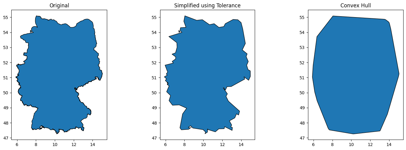
However, in the case of Germany, it leads to a gigantic 4Mb (!) GeoJSON file that drastically drags down the processing speed. I would strongly advise against using the exact geometry and would rather simplify it. You can use this code:

import osmnx as ox
import geopandas as gpd
import matplotlib.pyplot as plt
from shapely.geometry import Polygon

# Define the place of interest
place_name = "Germany"

# Get the boundary polygon using OSMnx
germany_boundary = ox.geocode_to_gdf(place_name)

# --- Simplification using tolerance ---
# a larger value will result in a more simplified polygon
tolerance = 0.1
simplified_germany_tolerance = germany_boundary.copy()
simplified_germany_tolerance["geometry"] = simplified_germany_tolerance.geometry.simplify(tolerance)

# --- Simplification using Convex Hull ---
simplified_germany_convex = germany_boundary.copy()
simplified_germany_convex["geometry"] = simplified_germany_convex.geometry.convex_hull

# --- Plotting ---

fig, axes = plt.subplots(1, 3, figsize=(15, 5))
germany_boundary.plot(ax=axes[0],  edgecolor='black', label="Original")
simplified_germany_tolerance.plot(ax=axes[1], edgecolor='black', label="Simplified using Tolerance")
simplified_germany_convex.plot(ax=axes[2], edgecolor='black', label="Convex Hull")

axes[0].set_title("Original")
axes[1].set_title("Simplified using Tolerance")
axes[2].set_title("Convex Hull")
plt.tight_layout()

plt.show()

# Save simplified version to geojson files
simplified_germany_tolerance.to_file("germany_simplified_tolerance.geojson", driver="GeoJSON")
simplified_germany_convex.to_file("germany_simplified_convex.geojson", driver="GeoJSON")

If you use the geometry that results from the file with a certain tolerance germany_simplified_tolerance.geojson, it takes only 45 seconds; using the convex hull only 33 seconds.

Httpfs/range requests compatible file formats

Now, there are different file formats that DuckDB can potentially read and that leverage httpfs/http range requests efficiently for very different purposes:

• Flatgeobuf is one of my favorites as it’s optimized for spatial retrieval of simple features by bounding boxes. It’s incredibly fast and you can use it very efficiently in lean web apps.

• Parquet is the swiss army knife of file formats and comes in handy everywhere. It does work for spatial purposes but is not as heavily optimized in this area as is Flatgeobuf. However, when it comes to column-based retrieval or complex filters, Parquet is likely to outshine Flatgeobuf.

• Mbtiles & Pmtiles are both used for vector tiles and complex geospatial features. Protomaps is a beautiful example of what can be achieved with just a single file (currently 120Gb for the entire world basemap) and some advanced engineering. It replaces a full tile server with just a single static file. The client requests the exact file chunks needed for a particular zoom level and bounding box and renders it with a style of your choice in the blink of an eye.

• COGs, so-called Cloud Optimized GeoTIFFs are the raster pendant to the above vector formats. They work similarly but focus on delivering efficient image delivery.

The are many more to add here, like of course SQLite with Spatiallite or Zarr.

Bonus: Geospatial Semantic Search

As you might guess, I am fascinated by these file formats. They replace heavy and costly server setups and are much more sustainable. And you can use them for (geospatial) semantic search too!

I understand Geospatial Semantic Search (GSS) as the user-driven process of employing semantic search to locate and rank similar documents to a user query on a map. Might sound easy but comes with a lot of tricky bananaskins that are not trivial to solve.

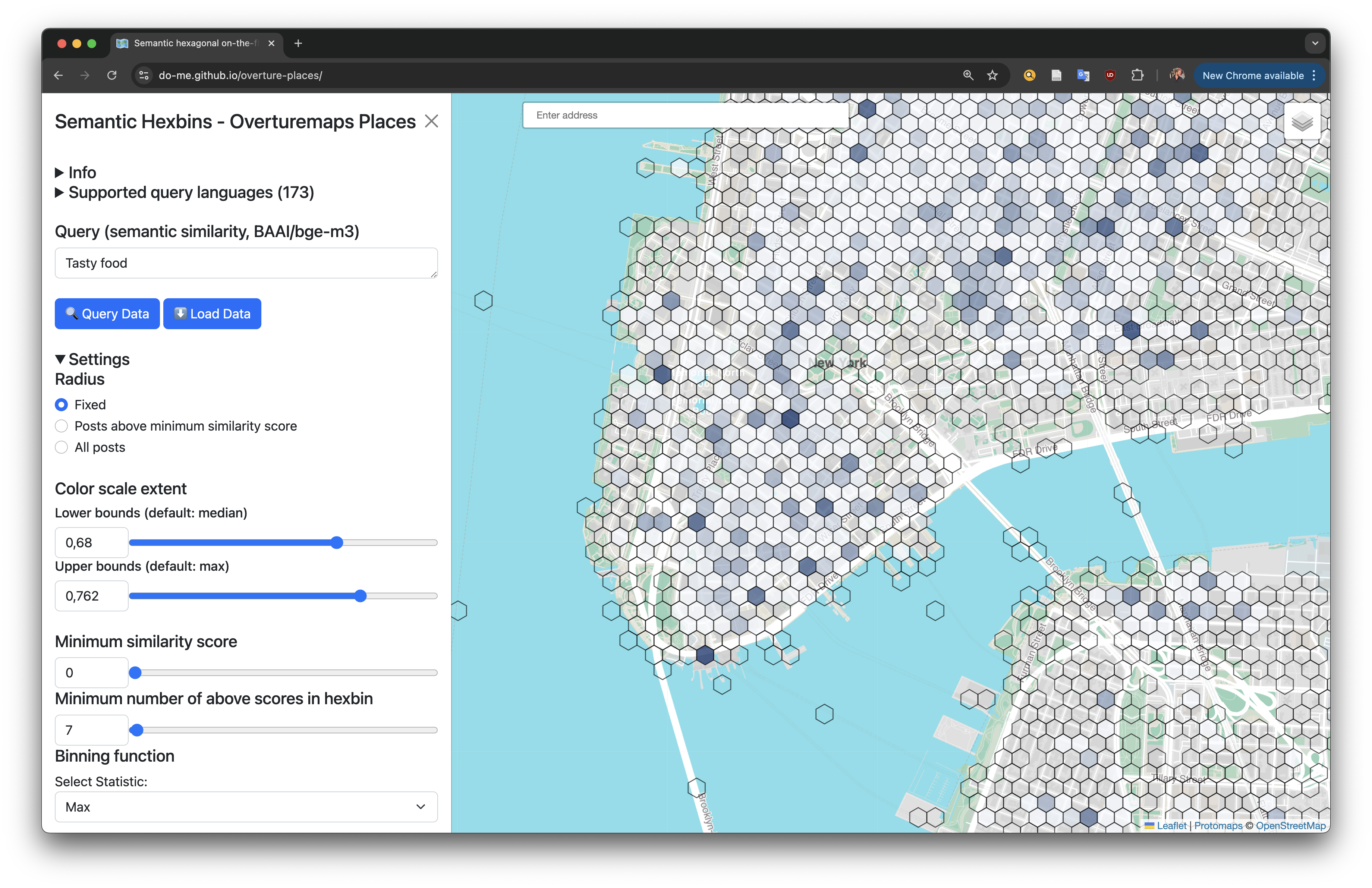
Based on Flatgeobuf, I created a single file for the Overture Places dump with bge-m3 embeddings for all the categories. In the frontend, a user can search anything in more than 100 languages (based on transformers.js) and gets a map with the most similar places. The entire app is hosted for free on Huggingface GitHub Pages. I will write a dedicated blog post about this workflow in the future.

You can try it yourself live here for your personal area of interest: https://do-me.github.io/overture-places/